Replicate STATA Robust Errors
Overview
In STATA, it’s good practice to estimate your OLS model with “robust” standard errors. For example, in STATA you type:
reg y x1 x2, r
And magic happens.
As it turns out, it’s not complete magic - it’s math. This post will recreate the robust standard error calculation using the free MATLAB clone, Octave. I’ll compare it to the same regressions run in STATA to verify.
TLDR: Here is a link to the full code to replicate yourself.
Problem
I’m going to assume that you have at least some basic familiarity with OLS regression or are learning about it right now. The setup is this: you have an outcome variable, Y, and some predictors, X (a.k.a. covariates, dependent variables), and you want to know which predictors are relevant to predict Y.
In order for the OLS to be the Best Linear Unbiased Estimator (BLUE), we need to believe - or assume - certain things about the “True” data generating process (DGP).
From Wooldridge, these are:
- Linear in parameters.
- Randomly sampled.
- There must be some variation in the dependent variables i.e. they can’t all be the same value.
- Zero conditional mean for the error term i.e. the expectation for the error should be zero, conditional on any values of
X. - Homoskedastic errors i.e. all errors come from the same distribution.
But what if we think the errors are not homoskedastic? In 1980, the economist Halbert White proposed a method for adjusting the standard errors to account for this possiblity.
Why do we care?
These standard errors are an input to the standard t-test, and therefore directly impact the interpretation of our point estimates for each parameter. If we don’t make this adjustment, we may draw incorrect conclusions about a variable’s importance.
Data
The first step is to make a good simulation dataset.
What we want
- A known “true” data generating process (DGP) so we can compare our results to the truth.
- Heteroskedastic deviations from the “truth” i.e. a given error’s variance depends on the observed independent variables.
How we make it
Ultimately, we will want to estimate a least-squared-error solution to:
\[Y = X\beta\]Here, \(Y\) is an \(N x 1\) column vector, \(X\) is an \(N x K\) matrix, and \(\beta\) is a \(K x 1\) vector. For the simulation, I’ll use 20 observations (i.e. \(N = 20\)), and three independent variables, including the constant / intercept (i.e. \(K = 3\)). The code for this is:
x1 = (1:n)';                       % e.g. "time" trend
x2 = round( randn(n, 1) * 10);     % e.g. random variable
c  = ones(n, 1);                   % the intercept

X = [x1 x2 c];
Next, we want to generate a vector of heteroskedastic errors i.e. the variance of the error changes, conditional on \(X\). I do this as follows:
u = randn(n, 1) .* x1 % randn ~ N(0, 1) so multiply by x1
Note that use of .* does element wise multiplication instead of matrix multiplication. In MATLAB and Octave, the same hold for any other operator e.g. .^ , ./ , etc. This multiplication ensures that the population variance changes, conditional on x.
Finally we are ready to make our outcome variable, \(y\). We will use the “true” data generating process (DGP) of:
\[y_i = 2 + 4x_{1i} - 3x_{2i}\]We do this in code, and add our heteroskedastic errors as follows:
truth = 2*c + 4*x1 - 3*x2;
Y     = truth + u;             % truth with errors
We save this, and will use it going forward.
Solution
Point estimates
We want to find coefficients that minimize the mean-squared-error. This is akin to saying we want coefficients that, on average, miss by as little as possible. In matrix notation we can say
\[min (Y - X\beta)' (Y - X\beta)\]One way to solve this is to take the derivative with respect to \(\beta\), and solve for \(\beta\).1 Doing so yields:
\[\beta = (X' X)^{-1} (X'Y)\]In MATLAB / Octave code, this takes the following form:
betas = inv(X' * X) * (X' * Y);
These will be our point estimates in a \(K x 1\) column vector.
Variance
We may wonder how confident we can be in those estimates. How precise are they? The “standard” way to estimate the standard error is to assume that all the “true” errors come from the same distribution (with the same variance). In this case we have residuals given by:
\[u = Y - X\beta\]And, under the homoskedastic error assumption, the variance is given by:
\[V(u_i | x_i) = E(u^2_i | x_i) = \sigma^2\]Whereas, under heteroskedastic errors, we assume:
\[V(u_i | x_i) = E(u^2_i | x_i) = \sigma^2_i\]Note that in this case, the variance of the error term can change with the values of \(x\): in other words, knowing \(x\) tells you something about how much you might miss by. If we think this is likely the case, we use the “robust” error calculation that follows.
Asymptotic Properties
Following certain “nice” assumptions,2 the estimates for β can be shown to come from the following asymptotic distribution:
\[\hat{\beta}_{OLS} \sim N \bigg(\beta, (X' X)^{-1} X' \Omega X (X' X)^{-1} \bigg)\]Where \(\Omega\) represents the variance-covariance matrix of the error terms. If the errors are homoskedastic, then we can let:
\[\Omega = \sigma^2I\]In practice, we can replace the theoretical population variance with the sum of the squared residuals, divided by the degrees of freedom. In code, this is:
% find residuals
resid = Y - X * betas;

% how many variables? need for degrees of freedom
k = size(X, 2);

% homoskedastic variance
s2 = sum( resid .^ 2) / (n - k);
stdVar = s2 * inv(X' * X);

% take element wise square-root to get error,
% only keep diagonal elements
stdErr = diag( stdVar .^ 0.5);
However, if the errors are heteroskedastic, then we have to allow the diagonal elements of \(\Omega\) to differ. In this case, White (1980) proposed to estimate it using the square of the estimated residuals.
In this case, our code becomes:
% take squared residuals and place in diagonal
omega = diag( resid .^ 2);

% calcualte adjusted "white" variance
whiteVar = inv(X'*X) * X'*omega*X * inv(X'*X) * (n/(n-k));

% keep only the diagonal elements and take square-root
whiteErr = diag( whiteVar .^ 0.5);
You might be wondering where the n/(n-k) came from - and that’s very observant of you. According to Cameron and Trivedi3, this convention to adjust by the degrees of freedom has limited theoretical basis, and is used out of convention and because simulation shows it works well. Go figure.
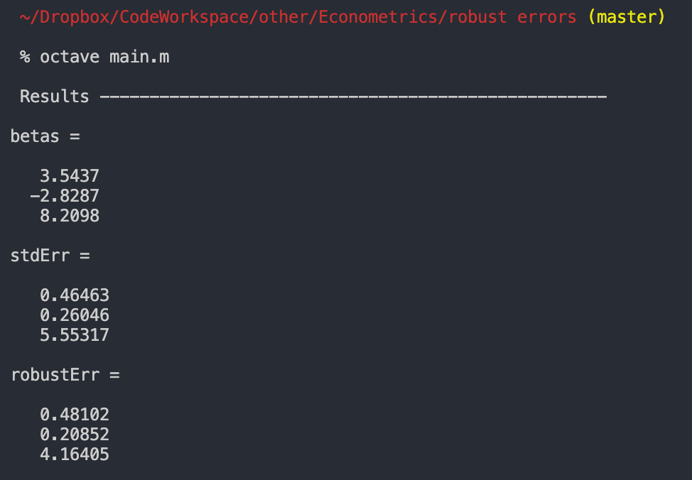
And we’re done! This code produces OLS estimates, standard errors, and “robust” standard errors that are consistent with STATA.
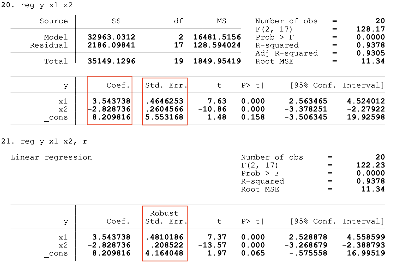
Verify with STATA
Now to the big question: does it work? See for yourself:
Full Code for Replication
The full code is available here on my GitHub for replication (and because it’s honestly easier to just see it all in one place and make sure it runs).