SEM Estimation by 2SLS

Overview

The goal is to:

1. Determine the correct setup for the first stage regression, and
2. Provide intuition for why that is the case.

Microeconomic Theory

Suppose the true supply function for some product is given by price, and one (or more) exogenous supply shifers \(Z_{supply}\). To make this concrete, consider the beef and steak products, where exogenous supply shifters would be inputs like the price of land, cattle feed, and so on.

and similarly, demand is given by:

If we observe transaction data in a competitive market, we will assume that prices and quantities are in equilibrium, thus implying:

and

Together, we can find the reduced form equation for the equilibrium values:

Similarly, we can solve equilibrium quantity as:

\(\textcolor{red}{NOTE}\): In equilibrium, price and quantity only depend on the exogenous supply and demand shifters.

Simulation

Using this theory as a guide, we can build a simulation dataset with the following linear functional forms:

Setup

and similarly, demand is given by:

Which gives us the reduced form relationships:

Where \(v = \frac{u_{demand} - u_{supply}}{2}\) contains the errors for both supply and demand.

Build Dataset

Using this relationship, we can create a simulation dataset as follows:

1. Generate random values for \(u_{demand}\), \(u_{supply}\), \(Z_{demand}\), and \(Z_{supply}\).
2. Use these to find equilibrium prices.
3. Back out equilibrium quantities from the supply or demand equation (and verify that they are in fact the same).
4. Finally, we only keep positive values for price and quantity since a firm would simply shut down if that were the case.

# number of observations to generate
N <- 100

# ud and us are exogenous ~ N(0, 1)
ud <- rnorm(N) 
us <- rnorm(N) 
v <- (ud - us) / 2

# supply and demand shifters are exogenous normal
# although I believe the distributional assumptions 
# can be relaxed
z1 <- rnorm(N) * 2 + 2  # ~N(2, 2)
z2 <- rnorm(N) + 3      # ~N(3, 0)

# price in equilibrium using reduced form equation
p <- 50 + z1 + z2 + v 

# verify quantities are the same in equilibrium!
qd <- 100 - p + 2*z2 + ud
qs <- p - 2*z1 + us
q  <- qd

if (sum(qd - qs) > 1e10) {
    cat("ERROR: Supply and demand not in equilibrium")
}

# make dataset 
# we only keep values where quantiy and price 
# are greater than zero. Our simulated datset may 
# contain negative values since non-zero conditions 
# are economic assumptions. 
data <- tibble(
        "Q" = q, 
        "P" = p, 
        "Z_Supply" = z1, 
        "Z_Demand" = z2
    ) %>% 
    filter(
        Q > 0 && P > 0
    )

Graph

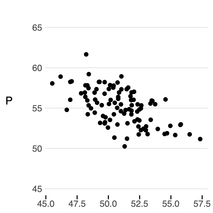
After generating a dataset according to those rules, we can view market prices and quantities in a scatter plot:

ymin <- min(data$P) - 5
ymax <- max(data$P) + 5
data %>% 
    ggplot(aes(Q, P)) + 
    geom_point() + 
    ylim(ymin, ymax) + 
    theme_wsj() 

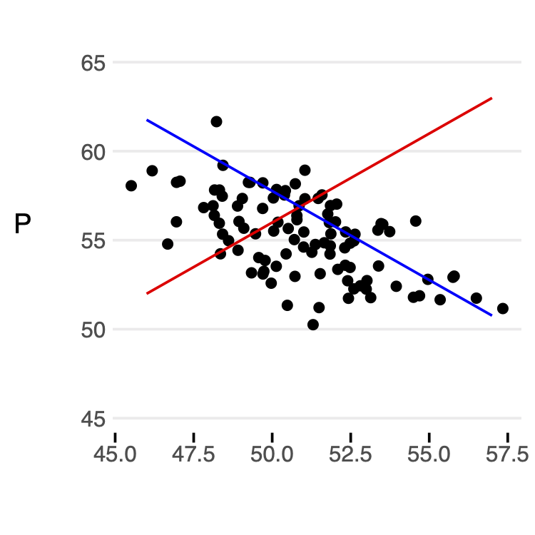
If we lock in some value of \(Z_{demand}\) and \(Z_{supply}\), we can easily see how supply and demand intersect.

z1_fixed1 <- data$Z_Supply[1]
z1_fixed2 <- data$Z_Supply[2]
z1_fixed3 <- data$Z_Supply[3]

z2_fixed1 <- data$Z_Demand[1]
z2_fixed2 <- data$Z_Demand[2]
z2_fixed3 <- data$Z_Demand[3]

data$Qs <- 1:dim(data)[1]
data$Ps1 <- data$Qs + 2 * z1_fixed1
data$Ps2 <- data$Qs + 2 * z1_fixed2
data$Ps3 <- data$Qs + 2 * z1_fixed3

data$Qd <- data$Qs
data$Pd1 <- 100 - data$Qd + 2 * z2_fixed1
data$Pd2 <- 100 - data$Qd + 2 * z2_fixed2
data$Pd3 <- 100 - data$Qd + 2 * z2_fixed3

xmin <- min(data$Q)
xmax <- max(data$Q)
ymin <- min(data$P) - 5
ymax <- max(data$P) + 5
data %>% 
    ggplot(aes(Q, P)) + 
    geom_point() + 
    geom_line(aes(Qs, Ps1), color = "red") + 
    geom_line(aes(Qd, Pd1), color = "blue") + 
    xlim(xmin, xmax) + 
    ylim(ymin, ymax) + 
    theme_wsj()

Intuition for First Stage

If we are trying to estimate demand elasticity by 2SLS, the naive regression of

We will get a biased estimate for \(\beta_1\). Intuitively, this is because price and quantity were determined in equilibrium. In other words, conditional on the exogenous supply and demand shifters (\(Z_{demand}\) and \(Z_{supply}\)), there is no variation in price or quantity.

Instead, we will rely on exogenous variation that only impacts quantity through supply, in this case the supply shifters \(Z_{supply}\). We can think of this as using exogenous shifts in the \(\textcolor{red}{red}\) line to help determine the slope of the \(\textcolor{blue}{blue}\) line.

data %>% 
    ggplot(aes(Q, P)) + 
    geom_point() + 
    geom_line(aes(Qs, Ps1), color = "red") + 
    geom_line(aes(Qs, Ps2), color = "red", linetype = "dashed") + 
    geom_line(aes(Qs, Ps3), color = "red", linetype = "dashed") + 
    geom_line(aes(Qd, Pd1), color = "blue") + 
    xlim(xmin, xmax) + 
    ylim(ymin, ymax) +
    theme_wsj() 

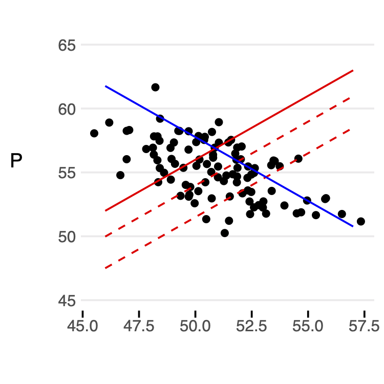
Finally, why is that that we include the demand shifters in the first equation? Intuitively, this helps to isolate which level of the curves we are looking at. For example, for a given supply curve, we still need to include demand factors to let us pinpoint where we expect the levels to intersect. In other words, we need to know the external factors that are affecting the \(\textcolor{red}{red}\) and \(\textcolor{blue}{blue}\) lines. As shown above, in equilibrium, those are the only factors for price and quantity.

Regression Results

Finally, we test these ideas directly to see if we can recover our original “true” demand parameters.

Recall, we are looking to retrieve the “true” values from the simulation setup,

Only Supply Shifters in First Stage

If we only include supply shifters in the first stage regression, i.e.

And use the predicted values, \(\hat{Q}\) in the second stage regression:

Then we obtain baised and inconsistent estimates. We can see the result of this estimation below:

# first stage 
first_stage_bias_fit <- lm(Q ~ Z_Supply, data = data)
data$`Q Predicted (only supply)` <- predict(first_stage_bias_fit)

# second stage 
fit_bias <- lm(P ~ `Q Predicted (only supply)` + Z_Demand, data = data)

We see here that these estimates are incorrect based on what we know to be true.

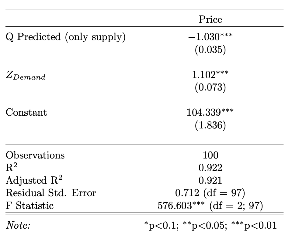
All Exogenous Variables in First Stage

If we now include all exogenous variables in the first stage regression, i.e.

And use these new predicted values, \(\widetilde{Q}\) in the second stage regression:

We can retrieve the known true paramater values.

# first stage 
first_stage_fit <- lm(Q ~ Z_Supply + Z_Demand, data = data)
data$`Q Predicted (all exogenous)` <- predict(first_stage_fit)

# second stage 
fit <- lm(P ~ `Q Predicted (all exogenous)` + Z_Demand, data = data)

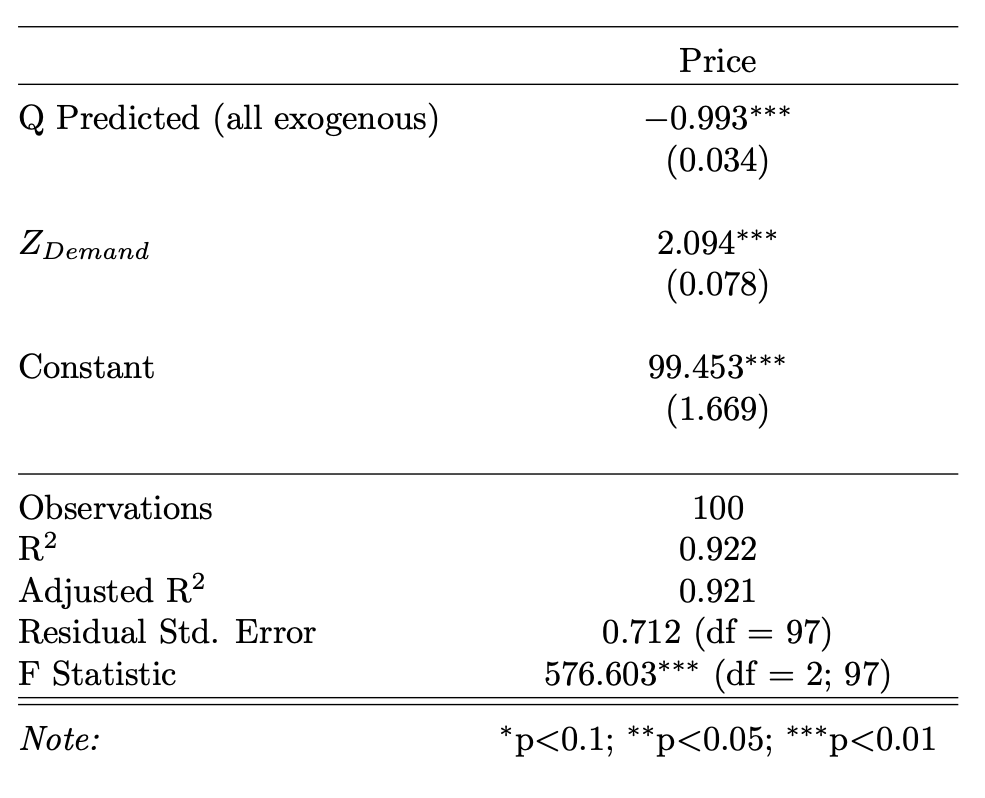
In this case, using all exogenous variables in the first stage allows us to recover the “true” demand parameters on quantity and the demand shifter.