Build a Neural Network with Julia

Audience

If you’re reading this, I assume you are already motivated to learn how a neural network actually works. They are relevant and powerful tools, so the sell shouldn’t be too difficult anyway. There are many other excellent guides out there that I will link to below. If you find any mistakes or have comments, please email me or comment on this post.

Introduction

I implement a feedforward, fully-connected neural network¹ with stochastic gradient descent in the Julia programming language (terms are defined below). There are two main advantages of this setup:

1. This architecture represents a neural network in its simplest feasible form.² Many other implementations, like convolutional or recurrant neural networks, are extensions of this base framework.

2. Julia is a fantastic language for learning this since it doesn’t distract from the math (i.e. matrix math is built in with convenient syntax), but still allows for powerful programming features that let us abstract from certain implementation details (i.e. using structs to create our own objects).

Note, this is for educational purposes only: it is (hopefully) optimized for readability rather than speed or scalability. For a production grade neural network in Julia, check out Flux.jl.

The full code is available here:

• https://github.com/slee981/neural-network.

Components and Definitions

• Neural Network: A sequence of mathematical operations, philosophically inspired by a model of the brain, and designed to iteratively improve its fit of historical data, while maintaining the ability to generalize to new, unseen data.
• Layer: A building block of a neural network that receives input, performs a basic linear (technically, affine) transformation, and passes the affine transformation through a non-linear “activation function” as its output.
• Feedforward: The forward process of receiving an input, and progressing through the network layer by layer until you reach the final output.
• Fully-connected: A type of neural network where each layer’s inputs are “connected” to the final output via its own potentially unique relationship i.e. no inputs are ignored, and no weights are systematically repeated.
• Affine Transformation: A geometric transformation that preserves lines and parallelism, but not necessarily distances and angles [source: Wikipedia]. For our use case, it is simply a transformation of the form \(z = Ax + b\). This technically differs from a linear transformation, since a linear transformation doesn’t have a “bias” component.
• Activation Function: A non-linear function applied element wise to a vector. Two common examples are the sigmoid and relu functions.
• Loss Function: A function that allows us to measure how well a predicted value matches the known “true” value. This is equivalently called a cost function.
• Stochastic Gradient Descent: An optimization process by which training a neural network is made feasible. Rather than calculating the true loss over the entire dataset before making a single update to our parameters, we only calculate the loss on a random subsample of the data and then update our weights accordingly. Emperically, this process is found to produce more general results as well as speed up the training process.

Big Picture

The goal of a neural network is to approximate a function, \(f(x)\), such that it is wrong as little as possible when it sees new data. We start with a training dataset containing \(N\) observations of \(k\) features (aka covariates), as well as \(N\) observations of some outcome that we will try to predict. For this exercise, I will ignore any use of a test dataset to focus on the math of the neural network.

We can conveniently store the features in an \(N\times k\) matrix called \(X\), and similarly store the outcomes in a matrix \(Y\). Thus, a length-\(k\) horizontal row vector \(x_i\) describes the features for observation \(i\) (for example, this could be a specific house, person, photo, or document depending on your data).

Visually, we can imagine this as follows:

Network

Together, the neural network acts to:

1. Receive an observation’s input, \(x_i\). This is the same as an individual row vector above, just transposed as a \(k \times 1\) column vector.
2. Take a linear (technically, affine) transformation of the input features, i.e. \(Ax_i + b\). Here, the matrix \(A\) has dimensions \(p \times k\), and the “bias” \(b\) is, accordingly, a \(p \times 1\) column vector.
3. Pass the resulting vector into a “non-linear activation function”, i.e. \(w_l = \sigma(Ax_i + b)\). The output here will be a \(p \times 1\) column vector.
4. Use this output vector, \(w_l\), as the input to the next layer and repeat the process until you reach the last layer.
5. Compare the last predicted output \(w_L\) to the observed target output \(y_i\) (using a loss function).
6. Calculate the gradient of the loss function with respect to the weights you can control in each layer, i.e. all \(A\)’s and \(b\)’s.
7. Update the weights in the direction of maximum change i.e. the negative gradient. This is what the commonly used names backpropagation and gradient descent refer to.
8. Repeat until satisfied.

Visually, we can represent the network as follows.

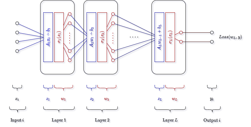
Note, this diagram is a bit different than the diagrams often shown. For me, this is more useful as it helps to internalize the fact that each layer is only performing basic math operations during the forward steps - no magic. Again, each layer will receive a vector of input, calculate a linear transformation (which returns another vector of possibly different length), pass each element of the new vector into a non-linear “activation” function, and then output that result to the next layer until there are no more layers.

Activation

We apply a non-linear “activation” function to the result of the linear transformation in order to allow the neural network to capture non-linear relationships. Conceptually, it is that simple.

Two very common activation functions are sigmoid and relu, defined as follows:

In this case, the activation function is applied element-wise to the linear transformation step, i.e.:

Without the activation function, \(\sigma\), the resulting series of linear tranasformations could be simplified to just a single simple linear transformation: we would never be able to fit more complex relationships. To convince youself this is true, consider the following example of a hypothetical three (3) layer network without an activation function:

Where we let \(A_s = A_3 A_2 A_1\) and \(b_s = A_3 A_2 b_1 + A_3 b_2 + b_3\). This simplification will hopefully convince you that an \(L\) layer neural network without a non-linear activation function applied to each of the layers will ultimately reduce to the mathematical equilivant of a single linear transformation.

If you need additional convincing, this Julia code will reproduce the above relationship:

x1 = randn(3, 1)

A1 = randn(4, 3)
A2 = randn(6, 4)
A3 = randn(2, 6)

b1 = randn(4, 1)
b2 = randn(6, 1)
b3 = randn(2, 1)

As = A3*A2*A1
bs = A3*A2*b1 + A3*b2 + b3

full       = A3*(A2*(A1*x1 + b1) + b2) + b3
simplified = As*x1 + bs

isapprox(full, simplified)
# true
#
# note: becuase of floating point precision
# the answers may be slightly different in the smallest decimal places
# which is why I use `isapprox`.

Loss

How do we evaluate success? Our neural network produces some output, and we may want to know how good that output is. You will hear this concept referred to as, equivalently, loss, cost, or objective functions.

The idea is simple: provide a way to quantify how good our model fits the data. In practice, this involves penalizing deviations from the true labeled results. If our model guesses the answer should be 0.21 when we know the answer is 1, we want the loss (cost) to be larger than if it had guessed 0.85.

In this write-up, I use the mean-squared-error loss function (largely due to the symmetry with standard OLS regression). There are other resources with great primers on other common loss functions, so I won’t cover it here. The important part is that we want to minimize the loss - and to do that we use calculus.

Backpropagation

Once we have made a guess at what the answer should be, \(w_L\), we compare it to the target output \(y_i\) and realize it may not be exactly correct. In this case our cost (loss) function \(C\) will produce a larger value than we want. How do we adjust the numbers in each layer’s weight matrix \(A_l\) and “bias”³ vector \(b_l\), such that the value of loss function will decrease i.e. our predicted output will be closer to the target output? We take derivatives.

In math, what we want to know is this: what is the partial derivative of the loss function with respect to each of the numbers I can control i.e. the elements of each weight matrix \(A_l\) and the bias vectors \(b_l\). Put another way, we want to find:

For each layer \(l \in [1, L]\). Important note: I will take some liberties with notation here to avoid additional superscripts and/or subscripts. Technically, a partial derivative must be taken with respect to a specific element, for example, \(\frac{\partial C}{\partial a_{ij}^l}\) for \(a_{ij}^l \in A_l\). In this case, I use notation that represents a “partial derivative of the cost function with respect to each of the elements of \(A_l\) and \(b_l\) in a layer”. Thus, the result of these family of derivatives I show will be vectors and matrices, rather than scalars.

To do so, we use a technique commonly called “backpropagation”, and also known as “reverse mode differentiation”.⁴ In short, rather than start from the input value and start chaining deravitives until you get to the output, we start with the output and work backwards to the input. This way, in one pass, we find all the relevant deravitives we care about. Check out the footnote in this paragraph for an excellent introduction to the concept.

Thus, starting with the last layer, we find deravitives:

It’s important to remember that we pick the relevant functions. So, for example, if we use a variant of the mean square error cost (loss) function we find

Note that when our target \(y_i\) is a vector instead of a scalar (e.g. for a categorical problem), we often choose a method of aggregating the losses for each element of that vector. In the Google framework Tensorflow, for example, they call this a reduction.⁵ The main reason for this is that it simplifies the math and calculations significantly. This simplification only applies to the reported “cost” (loss) value itself, not the derivative, however, which can remain a vector.

We can calculate the other necessary partial derivatives as well.

We can now put these values together to find our first relevant gradients (rearranging to fit the necessary geometry for matrix algebra):

More generally, using the chain rule, we can calculate the gradient for any layer as follows:

Actual implementations of these calculations can be found in the code below.

Stochastic Gradient Descent

Once we calculate how each of the numbers in our weights and biases impact the ultimate cost function, we need to decide how to update them such that the overall cost will decrease next time. For this, we use gradient descent. You may recall that the gradient points in the positive direction of maximum slope i.e. the gradient tells us, for a particular point in the space, which direction will a given change have the maximum impact. Since we are trying to minimize the cost function, we want to move in the negative direction of the same gradient vector: hence, gradient descent.

Since the gradient of the cost function is defined for the entire sample of \(N\) observations, in theory, we should have to do a forward pass of each data point in order to calculate the “true” loss. For large datasets, which we need for this type of machine learning, this becomes infeasible as you would need thousands and thousands of passes through the dataset.

Stochastic gradient descent is a heuristic solutions to this problem. Rather than calcualte the gradient of the cost function over the entire (training) dataset, we sample from our data and calculate the gradient over that subsample. This subsample can be as small as a single observation, and often isn’t more than 32 rows of data (i.e. observations).

Once we have our gradient, we update the weights according to some rule. The simplest takes the form:

Where \(u_{t+1}\) is the updated weight or bias, \(\eta\) acts as a scale for the update and is referred to as the step size or learning rate, and \(\nabla C(u_t)\) is the (stochastic) gradient of the cost function evaluated at the original point \(u_t\). To solidify this concept, we can imagine the gradient of the cost function looks something like:

Recalling, that the partial derivatives are calculated as above for each of the elements in the weight matricies \(A_l\) and bias vectors \(b_l\) for \(l \in [1, L]\). This is to say that, practically, we are calculating these elements backward from the last layer to the first layer

Implementation

We can implement the above with the Julia programming language. Ultimately, our goal is to call a neural network with the following interface:

net = Network(inputdim=input_size, cost=loss_mse, dcost=dloss_mse)
addlayer!(net, 64, relu, drelu) 
addlayer!(net, 32, relu, drelu) 
addlayer!(net, output_size, softmax, dsoftmax) 

# fit network - stochastic gradient descent 
fit!(net, X_train, Y_train, batchsize=16, epochs=10, learningrate=0.01)

Note, we will begin by defining the neural network with an input dimmension i.e. the length of each input vector. Subsequently, we add layers to the network by defining the size of the layer’s output, the activation function, and the derivative of the activation function⁶.

Network

First, we define a new “struct” in Julia, called Network:

mutable struct Network 
    inputdim::Int16
    layers::Vector{Layer}
    cost::Function
    dcost::Function

    # constructor
    function Network(;inputdim, cost, dcost)  
        new(inputdim, Array{Layer}[], cost, dcost)
    end
end

Julia notes:

• mutable struct .... If you’re unfamiliar with a “struct”, it’s a rather simple, but powerful, concept that shows up in other programming languages like C/C++ and Go. The idea is to group variables together in a way that is meaningful to the programmer or reader. With this, we can now create one or many new Networks and access the components with “dot” notation e.g. net.layers. The mutable keywork just allows us to modify the elements of the struct throughtout the program - by default, structs in Julia are immutable, and values don’t change after they are first created.
• var::Type. Julia allows for “type annotation”, which we’ll use define each variable a bit more precicely. In this case, the advantage is mostly for readability, and so that we know as best as possible what is happening each step of the way in our netural network. For example, when we see inputdim::Int16, it is simply saying that our network has a variable called inputdim that is a 16-bit integer. Similarly, cost::Function tells us (and the complier) to expect a function for the variable cost.
• function Network(;inputdim, cost, dcost). This is our “constructor”. It tells the compiler (and the programmer) how to create a new Network. For example, despite our Network having four internal variables, we create a new network with only three input arguments (because we don’t have any layers yet). One final note - the semicolon “;” before inputdim forces us to explicitly declare the variable we’re setting, rather than rely on the position. So we can create a new network with net = Network(inputdim=4, cost=mse, dcost=dmse), but if we try to say net = Network(4, mse, dmse) the compiler will throw an error. This is a design choice by me, feel free to remove it for your use.

Layer

Next, we define a new struct for each Layer:

mutable struct Layer
    weights::AbstractArray
    bias::AbstractArray

    # each layer can have its own activation function
    activation::Function
    dactivation::Function

    # cache 
    # 1- the last linear transformation: z = Ax + b
    # 2- activated output: w = activation(z) 
    linear_out::AbstractArray
    activated_out::AbstractArray

    # keep track of partial derivative error for each batch 
    dC_dlinear::AbstractArray 
    dC_dweights::AbstractArray 
    dC_dbias::AbstractArray 

    # constructor
    function Layer(
        insize::Number, 
        outsize::Number, 
        activation::Function, 
        dactivation::Function)

        # the Glorot normal initializer, also called Xavier normal initializer
        #
        # reference: 
        # https://github.com/tensorflow/tensorflow/blob/master/tensorflow/python/keras/initializers/initializers_v2.py
        sigma_sq = 2 / (insize + outsize)
        weights = randn(outsize, insize) * sigma_sq
        bias = randn(outsize, 1) * sigma_sq

        linear_out = zeros(outsize, 1)
        activated_out = zeros(outsize, 1)

        dC_dlinear = zeros(outsize, 1)
        dC_dweights = zeros(outsize, insize)
        dC_dbias = zeros(outsize, 1)
        new(weights, bias, activation, dactivation, linear_out, activated_out, dC_dlinear, dC_dweights, dC_dbias)
    end
end

Julia note:

• Similar to the Network above, we create a new mutable struct to represent a Layer. One practical note is that we use AbstractArray because it allows us to set those variables as either a one-dimensional vector, or two-dimensional matrix. This works because of type inheritance, which is worth reading about in the official Julia documentation.

Network note:

• Each layer will store information about its current weights and biases, as well as its activation function and the derivative.
• Additionally, each layer will store some values for the backpropagation step. Namely, we will keep track of the last output for both the linear and “activated” vectors, as well as the running total of the various relevant partial derivatives i.e. the partial derivative of the cost (loss) function with respect to the linear transformation \(z\), the weights \(A\), and the bias vector \(b\).

Initializing the Layer

When we create a new layer, we need to make a decision about how to initialize the weights and bias. Zeros are not a good choice, because our first forward passes will be uninteresting (the result is the same for all input), and it will be difficult to update during backpropagation. Thus, we want to initialize the weights and bias with some random component, the specifics of which we follow the default setting in Google’s Tensorflow and use a so-called Glorot normal. This process basically allows us to initialize the weights and bias from a normal distribution with mean zero, and a variance that depends on the size of the inputs and outputs.

Besides that, we set all of the “cache” values equal to zeros, since they will be calculated in due time.

Feedforward

For each step, we need to make a forward pass of the network, which is a fancy way of saying we need to take an input \(x\) and transform it to an output \(w_L\).

function feedforward!(net::Network, input::AbstractArray)::AbstractArray
    nlayers = length(net.layers)

    lastoutput = input 
    for i = 1:nlayers
        layer = net.layers[i]

        # linear_out: z = Ax + b 
        layer.linear_out = layer.weights * lastoutput + layer.bias

        # activated_output: w = activation(Ax + b)
        layer.activated_out = layer.activation(layer.linear_out)

        # update for the next input
        lastoutput = layer.activated_out 
    end

    # w_L
    return lastoutput
end

This code should be pretty simple: starting with the input, for each layer in the network, calculate the linear transformation \(z = Ax + b\), the activated transformation \(w = \sigma(z)\), and then use the previous layer’s output as input to the next layer.

Julia note:

• By convention, when a function can modify the element it’s being passed, we include an exclaimation mark “!” at the end of the function i.e. feedforward! as opposed to feedforward. This is related to a paradigm called “pass by reference” in which you allow the function to modify the actual object you passed it. In contrast, “pass by value” will make a copy of the object’s value, do some operation, and return a new value. Both are useful, and Julia allows for both. In this case, we want these functions to directly update the actual network.
• Additionally, just like type annotation with variables, in Julia we can give the compiler (and the programmer) a hint that this function returns a value of type AbstractArray. We signify that by fctname()::ReturnType.

Backpropagation

Based on our understanding with the big picture above, backpropagation is perhaps more aptly named “calculate partial derivatives”. One key note is that we will keep a running total of the partial derivatives for each input until we are ready to actually use them to update the weights and bias. The batch size of our stochastic gradient descent will tell us how many inputs the network will “see” before updating the weights.

function backpropagate!(net::Network, x::AbstractArray, truth::AbstractArray)

    # calculate last layer partials 
    lastlayer = net.layers[end]

    lastlayer.dC_dlinear   = lastlayer.dactivation(lastlayer.linear_out) * net.dcost(lastlayer.activated_out, truth)
    lastlayer.dC_dweights += lastlayer.dC_dlinear * net.layers[end - 1].activated_out'
    lastlayer.dC_dbias    += lastlayer.dC_dlinear

    # iterate through previous layer partials
    # note arrays are indexed at 1, not 0
    for i = 1:(length(net.layers) - 1)
        layer     = net.layers[end - i]      # layer "l"
        nextlayer = net.layers[end - i + 1]  # nextlayer "l + 1"

        # select the output of the previous layer
        # note, for the first layer this will be the original input, xi
        if i + 1 < length(net.layers)
            prevlayer = net.layers[end - i - 1]
            prevout   = prevlayer.activated_out

        elseif i + 1 == length(net.layers)
            prevout = x
        end

        layer.dC_dlinear   = layer.dactivation(layer.linear_out) * nextlayer.weights' * nextlayer.dC_dlinear 
        layer.dC_dweights += layer.dC_dlinear * prevout'
        layer.dC_dbias    += layer.dC_dlinear 
    end
end

Stochastic Gradient Descent

Putting it all together, our stochastic gradient descent step breaks the input data into separate batches, and performs the forward pass, the backpropagation, and updates the weights according to the batch size. Together, we see:

function sgd!(
    net::Network, 
    x::AbstractArray, 
    y::AbstractArray, 
    batchsize::Number, 
    epochs::Number, 
    learningrate::Number)
    # stochastic gradient descent (sgd)

    # input vars
    nobs, nvars = size(x)

    # how many times do we go through the dataset? 
    for epoch = 1:epochs

        # shuffle rows of matrix  
        shuffledrows = shuffle(1:nobs)
        x = x[shuffledrows, :]
        y = y[shuffledrows, :]

        # track average losses for each sample in batch
        losses = Vector{Number}();

        # create mini batches and loop through each batch 
        # note: julia is NOT zero indexed 
        #       i.e. x[1] is the first element
        for batchend = batchsize:batchsize:nobs
            batchstart = batchend - batchsize + 1

            # get sample of rows i.e. observations 
            # and transpose into columns for feedforward
            xbatch = x[batchstart:batchend, :]'
            ybatch = y[batchstart:batchend, :]'

            for icol in 1:batchsize
                xi    = xbatch[:, icol:icol]
                ytrue = ybatch[:, icol:icol]

                # feedforward
                out = feedforward!(net, xi)

                # calculate loss and store for tracking progress
                iloss = net.cost(out, ytrue)
                push!(losses, iloss)

                # calculate partial derivatives of each weight and bias
                # i.e. backpropagate
                backpropagate!(net, xi, ytrue)
            end

            # update weights and bias 
            update!(net, learningrate)
        end

        # sample average loss from batch to track progress
        push!(epochlosses, mean(losses))
    end
end

And note that each update step on the network adjusts the weights and biases as follows:

function update!(net::Network, learningrate::Number)

    # update weights in each layer based on the error terms dC_dweights, dC_dbias
    for i = 1:length(net.layers)
        layer = net.layers[i]

        # gradient descent step 
        layer.weights -= learningrate * layer.dC_dweights
        layer.bias    -= learningrate * layer.dC_dbias

        # reset the error terms for next batch 
        nrows, ncols = size(layer.weights)

        layer.dC_dlinear  = zeros(nrows, 1)
        layer.dC_dweights = zeros(nrows, ncols)
        layer.dC_dbias    = zeros(nrows, 1)
    end
end

Conclusion

That concludes the basics. The full code is available here:

• https://github.com/slee981/neural-network.

For me, the key takeaways from this exercise are:

1. Neural networks are intricate combinations of math, but not magic.
2. The complex layering of weights, biases, and activation functions makes interpretation very challenging, if not useless. This is to suggest that neural networks are fantastic at fitting data, but that reverse engineering why or how the neural network arrives at a given answer is beyond the scope of our current tool kit.

The implications of this are to consider when a neural network is the right tool for the job, and when it might not be.

For example, I suspect many people would be uneasy with the Federal Reserve setting the interest rate based on predictions from a neural network. Rather, Reserve Bank presidents and their teams of researchers have an (implicit or explicit) responsibilty to explain to congress, and the American people, why they made their decision. Much effort goes into these written and verbal explainations, and much effort occurs behind the scenes to estimate the implications of their decisions through the lens of cause and effect.

Alternatively, a neural network’s tremendous power at fitting patterns in data is perfectly geared to other problems, for example, image recognition for a search engine, or foreign language translation. In these cases, there is much less emphasis on why and much more emphasis on what or which.

Thus, these different questions we ask ourselves may require different tools: in some cases, prediction alone may not be all that we are after.

Resources

1. Learning From Data, Gilbert Strang: http://math.mit.edu/~gs/learningfromdata/
2. Michael Nielsen’s “Neural Networks and Deep Learning”: http://neuralnetworksanddeeplearning.com/
3. Blog post on computational graphs: https://colah.github.io/posts/2015-08-Backprop/.

Footnotes